import pandas as pd
import seaborn as sns
import matplotlib.pyplot as plt
import numpy as np
import re
%matplotlib inlineOKCupid Date-A-Scientist
Python
Machine learning
NLP
EDA
Using EDA and supervised machine learning to test whether an OKCupid user’s zodiac sign can be predicted (spoiler: it can’t).
Introduction
In recent years, there has been a massive rise in the usage of dating apps to find love. Many of these apps use sophisticated data science techniques to recommend possible romantic matches and optimize the user experience. These apps give us access to a wealth of information that we’ve never had before about how different people experience romance.
Scope
This project utilises information from dating platform OkCupid 1 in order to answer specific problems.
Project Goals
There are two primary goals for this project. The first is to perform EDA - scoping, initial analysis and investigation) on the data, which will then be cleaned and prepared for use in several supervised machine learning algorithms. The second goal is to use this data to see if it is possible to determine the zodiac sign of a OkCupid member, using the information provided in their profile. Zodiac signs have been identified as an important attribute in the dating world, and as a portion of profiles do not provide this information, it would be useful for OkCupid to predict missing zodiac signs, in order to increase the likelihood of successful dating matches.
Data
The data is included within profiles.csv, which has been provided by Codecademy 2. T The data contains 59946 rows (each representing an individual OkCupid user) and 31 columns. The columns contain information about the age, body type, diet, alcohol and drug consumption, education level, job and income, ethnicity, height, children and pets, sexual orientation, sex, zodiac sign and spoken languages as well as answers to several multiple choice or short-essay style questions.
Analysis
Visualisation and descriptive statistical methods will be used to understand the data, before building and applying four supervised machine learning classification algorithms: - Linear regression - K-nearest neighbors - Random forest - NLP/Naive Bayes
Results and Evaluation
The results of the machine learning algorithms will be reported and their success levels evaluated. Following this, recommendations for improved results and next steps will be discussed.
Importing the data
Importing libraries
Loading the dataframe
okc = pd.read_csv(r'profiles.csv')
(okc.head(5))| age | body_type | diet | drinks | drugs | education | essay0 | essay1 | essay2 | essay3 | ... | location | offspring | orientation | pets | religion | sex | sign | smokes | speaks | status | |
|---|---|---|---|---|---|---|---|---|---|---|---|---|---|---|---|---|---|---|---|---|---|
| 0 | 22 | a little extra | strictly anything | socially | never | working on college/university | about me:<br />\n<br />\ni would love to think... | currently working as an international agent fo... | making people laugh.<br />\nranting about a go... | the way i look. i am a six foot half asian, ha... | ... | south san francisco, california | doesn’t have kids, but might want them | straight | likes dogs and likes cats | agnosticism and very serious about it | m | gemini | sometimes | english | single |
| 1 | 35 | average | mostly other | often | sometimes | working on space camp | i am a chef: this is what that means.<br />\n1... | dedicating everyday to being an unbelievable b... | being silly. having ridiculous amonts of fun w... | NaN | ... | oakland, california | doesn’t have kids, but might want them | straight | likes dogs and likes cats | agnosticism but not too serious about it | m | cancer | no | english (fluently), spanish (poorly), french (... | single |
| 2 | 38 | thin | anything | socially | NaN | graduated from masters program | i'm not ashamed of much, but writing public te... | i make nerdy software for musicians, artists, ... | improvising in different contexts. alternating... | my large jaw and large glasses are the physica... | ... | san francisco, california | NaN | straight | has cats | NaN | m | pisces but it doesn’t matter | no | english, french, c++ | available |
| 3 | 23 | thin | vegetarian | socially | NaN | working on college/university | i work in a library and go to school. . . | reading things written by old dead people | playing synthesizers and organizing books acco... | socially awkward but i do my best | ... | berkeley, california | doesn’t want kids | straight | likes cats | NaN | m | pisces | no | english, german (poorly) | single |
| 4 | 29 | athletic | NaN | socially | never | graduated from college/university | hey how's it going? currently vague on the pro... | work work work work + play | creating imagery to look at:<br />\nhttp://bag... | i smile a lot and my inquisitive nature | ... | san francisco, california | NaN | straight | likes dogs and likes cats | NaN | m | aquarius | no | english | single |
5 rows × 31 columns
#print(okc.columns)
#print(okc.dtypes)
(okc.info())
print(f"Number of rows = {len(okc.age)}")
<class 'pandas.core.frame.DataFrame'>
RangeIndex: 59946 entries, 0 to 59945
Data columns (total 31 columns):
# Column Non-Null Count Dtype
--- ------ -------------- -----
0 age 59946 non-null int64
1 body_type 54650 non-null object
2 diet 35551 non-null object
3 drinks 56961 non-null object
4 drugs 45866 non-null object
5 education 53318 non-null object
6 essay0 54458 non-null object
7 essay1 52374 non-null object
8 essay2 50308 non-null object
9 essay3 48470 non-null object
10 essay4 49409 non-null object
11 essay5 49096 non-null object
12 essay6 46175 non-null object
13 essay7 47495 non-null object
14 essay8 40721 non-null object
15 essay9 47343 non-null object
16 ethnicity 54266 non-null object
17 height 59943 non-null float64
18 income 59946 non-null int64
19 job 51748 non-null object
20 last_online 59946 non-null object
21 location 59946 non-null object
22 offspring 24385 non-null object
23 orientation 59946 non-null object
24 pets 40025 non-null object
25 religion 39720 non-null object
26 sex 59946 non-null object
27 sign 48890 non-null object
28 smokes 54434 non-null object
29 speaks 59896 non-null object
30 status 59946 non-null object
dtypes: float64(1), int64(2), object(28)
memory usage: 14.2+ MB
Number of rows = 59946The data provided has the following columns, which provide multiple choice answers:
- body_type - categorical variable
- diet - categorical variable
- drinks - categorical variable
- drugs - categorical variable
- education - categorical variable
- ethnicity - categorical variable
- height - continuous variable
- income - continuous variable
- job - categorical variable
- last_online - date variable
- offspring - categorical variable
- orientation - categorical variable
- pets - categorical variable
- religion - categorical variable
- sex - categorical variable
- sign - categorical variable
- smokes - categorical variable
- speaks - categorical variable
- status - categorical variable
And a set of open short-answer responses to :
- essay0 - My self-summary
- essay1 - What I’m doing with my life
- essay2 - I’m really good at…
- essay3 - The first thing people usually notice about me…
- essay4 - Favorite books, movies, show, music, and food
- essay5 - The six things I could never do without
- essay6 - I spend a lot of time thinking about…
- essay7 - On a typical Friday night I am…
- essay8 - The most private thing I am willing to admit
- essay9 - You should message me if…
Changing the essay question columns into easier to understand variable names
okc.rename(columns={'essay0' : 'self_summary', 'essay1' : 'life_plans', 'essay2': 'good_at', 'essay3' : 'notice_about', 'essay4' : 'favourites', 'essay5' : 'do_without', 'essay6' : 'think_about', 'essay7' : 'friday', 'essay8' : 'private', 'essay9' : 'message'}, inplace=True)
(okc.columns)
Index(['age', 'body_type', 'diet', 'drinks', 'drugs', 'education',
'self_summary', 'life_plans', 'good_at', 'notice_about', 'favourites',
'do_without', 'think_about', 'friday', 'private', 'message',
'ethnicity', 'height', 'income', 'job', 'last_online', 'location',
'offspring', 'orientation', 'pets', 'religion', 'sex', 'sign', 'smokes',
'speaks', 'status'],
dtype='object')An initial brief look at the numerical data within the dataframe
(okc.describe())| age | height | income | |
|---|---|---|---|
| count | 59946.000000 | 59943.000000 | 59946.000000 |
| mean | 32.340290 | 68.295281 | 20033.222534 |
| std | 9.452779 | 3.994803 | 97346.192104 |
| min | 18.000000 | 1.000000 | -1.000000 |
| 25% | 26.000000 | 66.000000 | -1.000000 |
| 50% | 30.000000 | 68.000000 | -1.000000 |
| 75% | 37.000000 | 71.000000 | -1.000000 |
| max | 110.000000 | 95.000000 | 1000000.000000 |
Exploring the data
Zodiac signs
First we will take a look at the zodiac sign data within the dataframe.
okc.sign.nunique()48There appears to be 48 answers to the ‘What is your zodiac sign?’ question. As there are only 12 possible signs, this data must be looked at more closely.
okc.sign.unique()array(['gemini', 'cancer', 'pisces but it doesn’t matter', 'pisces',
'aquarius', 'taurus', 'virgo', 'sagittarius',
'gemini but it doesn’t matter',
'cancer but it doesn’t matter',
'leo but it doesn’t matter', nan,
'aquarius but it doesn’t matter',
'aries and it’s fun to think about',
'libra but it doesn’t matter',
'pisces and it’s fun to think about', 'libra',
'taurus but it doesn’t matter',
'sagittarius but it doesn’t matter',
'scorpio and it matters a lot',
'gemini and it’s fun to think about',
'leo and it’s fun to think about',
'cancer and it’s fun to think about',
'libra and it’s fun to think about',
'aquarius and it’s fun to think about',
'virgo but it doesn’t matter',
'scorpio and it’s fun to think about',
'capricorn but it doesn’t matter', 'scorpio',
'capricorn and it’s fun to think about', 'leo',
'aries but it doesn’t matter', 'aries',
'scorpio but it doesn’t matter',
'sagittarius and it’s fun to think about',
'libra and it matters a lot',
'taurus and it’s fun to think about',
'leo and it matters a lot',
'virgo and it’s fun to think about',
'cancer and it matters a lot', 'capricorn',
'pisces and it matters a lot', 'aries and it matters a lot',
'capricorn and it matters a lot', 'aquarius and it matters a lot',
'sagittarius and it matters a lot', 'gemini and it matters a lot',
'taurus and it matters a lot', 'virgo and it matters a lot'],
dtype=object)The signs are quantified with the importance of zodiac signs to an OkCupid user. Whilst this is interesting information, intially it is best to remove this data and place the cleaned zodiac sign in a new column. Creating a new column means the sign importance data is retained for future use, if required.
okc['sign_clean']= okc.sign.str.split(' ').str[0]
okc.sign_clean.nunique()
sign_labels = list(okc.sign_clean.unique())
sign_labels_nonull = [item for item in sign_labels if not(pd.isnull(item)) == True]
print(sign_labels_nonull)

sign_labels_plt = [x.title() for x in sign_labels_nonull]
print(sign_labels_plt)
['gemini', 'cancer', 'pisces', 'aquarius', 'taurus', 'virgo', 'sagittarius', 'leo', 'aries', 'libra', 'scorpio', 'capricorn']
['Gemini', 'Cancer', 'Pisces', 'Aquarius', 'Taurus', 'Virgo', 'Sagittarius', 'Leo', 'Aries', 'Libra', 'Scorpio', 'Capricorn']The 12 unique zodiac signs are now correctly labelled in the okc.sign_clean column and the spread is represented in the plot below. The data appears fairly balanced, with capricorn representing slightly less of the users.
sns.set(style = 'ticks')
sns.set_context("notebook", font_scale=1.2, rc={"lines.linewidth": 2.5})
f, ax = plt.subplots(figsize=(15,8))
sns.countplot(data=okc, y='sign_clean')
sns.color_palette("Spectral", as_cmap=True)
ax.set_ylabel('')
ax.set_xlabel('Count')
ax.set_title('Proportion of zodiac signs in the OkCupid data')
ax.set_yticklabels(sign_labels_plt)
plt.show()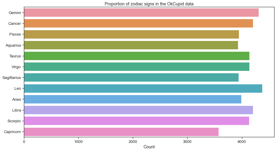
Continuous variables
Now we have looked at the zodiac sign data, let’s explore the data that will be used to predict zodiac signs.
Age range
sns.set_style('ticks')
#sns.set_context('notebook')
sns.set_context("notebook", font_scale=1.5, rc={"lines.linewidth": 2.5})
f, (ax1, ax2) = plt.subplots(1,2, sharey=False, figsize=(12,6))
plt.subplots_adjust(wspace=0.5)
ax1 = sns.histplot(okc.age, color='purple', ax=ax1)
ax1.set_title('Age distribution of OkCupid profiles')
ax1.set_xlabel('Age')
ax2 = sns.histplot(okc.age[okc.age > 50], color='pink', ax=ax2)
ax2.set_title('Age distribution of profiles above 50 years old')
ax2.set_xlabel('Age')
plt.show()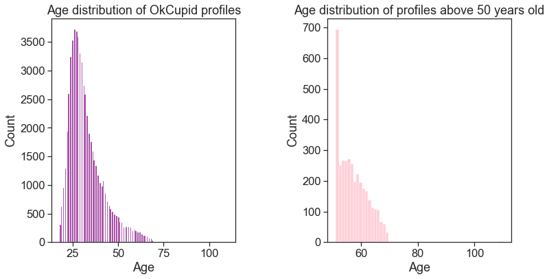
print(f'Mean age: {round(okc.age.mean(), 2)} ')
print(f'90th percentile: {okc.age.quantile(0.9)}')
print(f'Maximum age: {okc.age.max()} ')
print(f'Minimum age: {okc.age.min()} ')
Mean age: 32.34
90th percentile: 46.0
Maximum age: 110
Minimum age: 18 The mean age of users is 32 years old, with 90% of the data lying below 46 years. The maximum age is 110, which is either impressive, someone didn’t want to disclose their age, or is an error. This outlier causes the already left-skewed data to be further skewed. Therefore, the two outliers, at 109 and 110, are best removed in order to minimise their effect on the total distribution of the data, and thus the statistical analysis.
okc = okc[okc.age < 75]
sns.set_style('ticks')
#sns.set_context('notebook')
sns.set_context("notebook", font_scale=1.5, rc={"lines.linewidth": 2.5})
sns.displot(data=okc, x="age", hue="sex", multiple = "stack", palette=['blue', 'red'], kind='hist', binwidth=2)
plt.title('Age distribution of OkCupid profiles of both sexes')
plt.xlabel('Age')
plt.show()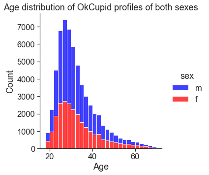
The plot shows that the age distribution for males and females is very similar - but also indicates that more males than females use OkCupid.
Height
#collapse-output
print(okc.height.value_counts())
70.0 6074
68.0 5449
67.0 5353
72.0 5315
69.0 5179
71.0 4826
66.0 4759
64.0 3865
65.0 3794
73.0 2815
63.0 2767
74.0 2547
62.0 2244
75.0 1382
61.0 1090
60.0 791
76.0 783
77.0 280
59.0 212
78.0 132
79.0 57
58.0 53
80.0 27
95.0 19
57.0 17
83.0 12
81.0 11
82.0 11
36.0 11
84.0 9
56.0 8
55.0 6
53.0 5
94.0 3
54.0 3
91.0 3
50.0 2
88.0 2
37.0 2
48.0 2
43.0 2
1.0 1
51.0 1
90.0 1
26.0 1
85.0 1
9.0 1
89.0 1
92.0 1
87.0 1
49.0 1
47.0 1
6.0 1
42.0 1
86.0 1
3.0 1
8.0 1
93.0 1
52.0 1
4.0 1
Name: height, dtype: int64fig, (ax1) = plt.subplots(figsize=(7, 6))
sns.set_style('ticks')
#sns.set_context('notebook')
sns.set_context("notebook", font_scale=1.5, rc={"lines.linewidth": 2.5})
sns.histplot(data=okc, x="height", hue="sex", binwidth=2, multiple = "stack", palette=['blue', 'red'], ax=ax1)
ax1.set_xlim(55, 85)
plt.title('Height distribution of OkCupid users')
plt.xlabel('Height')
plt.show()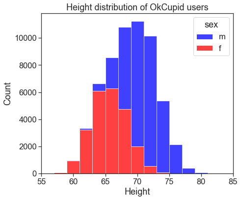
print(f'Minimum female height: {okc.height[okc.sex == "f"].min()} inches')
print(f'Minimum male height: {okc.height[okc.sex == "m"].min()} inches')
print(f'Maximum female height: {okc.height[okc.sex == "f"].max()} inches')
print(f'Maximum female height: {okc.height[okc.sex == "m"].max()} inches')
print(f'Average female height: {round(okc.height[okc.sex == "f"].mean(),2)} inches')
print(f'Average male height: {round(okc.height[okc.sex == "m"].mean(),2)} inches')
Minimum female height: 4.0 inches
Minimum male height: 1.0 inches
Maximum female height: 95.0 inches
Maximum female height: 95.0 inches
Average female height: 65.1 inches
Average male height: 70.44 inchesThe minimum heights listed are 4 inches and 1 inches for females and males, respectively. We can assume that people did not want to list their height in their profiles. As heights for both males and females are normally distributed the small values will not be removed - perhaps a certain zodiac sign prefers not to disclose their height. The average height for females is 65 inches, or 5ft 5in and the average height for males is 5ft 10.5in.
Income
sns.displot(okc.income, color='green')
sns.set_style('ticks')
#sns.set_context('notebook')
sns.set_context("notebook", font_scale=1.5, rc={"lines.linewidth": 2.5})
plt.title('Distribution of income for OkCupid profiles')
plt.xlabel('Income')
plt.show()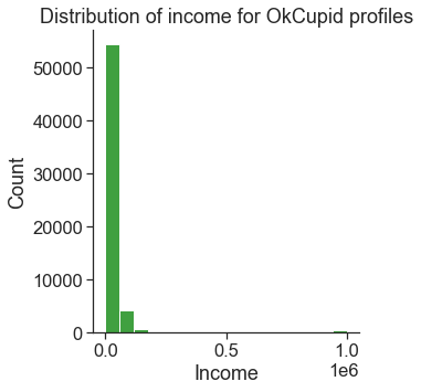
okc_no_income =(okc.income == -1).value_counts()
percent_no_income = (okc_no_income[1] / (okc_no_income[0] + okc_no_income[1])) * 100

print(okc_no_income)
print(percent_no_income)
True 48440
False 11504
Name: income, dtype: int64
80.80875483784867It appears that most people, 81 %, prefer not to disclose their income in their dating profile. This could be for several reasons, such as it is often seen as crass to discuss income, or that people do not want money to be a factor in choosing a date. Given this lack of information, income will not be considered when applying models to the data.
Discrete variables
Now we have looked at the continuous variables above, the next section will discuss the discrete variables, which make up the majority of the data.
Sex
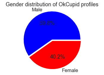
The sex distribution of the OkCupid profiles shows that there is a larger proportion of males to females. The data does not include any trans or non-binary labels, which could indicate that perhaps the profiles in the data did not include these groups, only binary options were available or only sex at birth were considered.
plt.pie(okc.sex.value_counts(), labels=['Male', 'Female'], colors=['blue', 'red'], autopct='%0.1f%%', explode=[0.02]*2)
plt.axis('equal')
plt.title('Gender distribution of OkCupid profiles')
plt.show()
# function for plotting countplots to investigate the variables
def plotting_tool(df, x, width, height):
    sns.set_style('ticks')
    sns.set_context("notebook", font_scale=1.5, rc={"lines.linewidth": 2.5})
    sns.color_palette("Spectral", as_cmap=True)
    plt.figure(figsize=[width, height])
    plt.subplots_adjust(wspace=0.5, hspace=0.3)
    for i in range(len(x)):
            plt.subplot(1, len(x), i+1)
            sns.countplot(data=df, y=x[i])
            sns.color_palette("Spectral", as_cmap=True)
            plt.title(f'{x[i]}')
            plt.ylabel('')
            plt.xlabel('Count')
Diet and body
OkCupid users can list their body type and diet choices in their profiles. The diet answers have qualifying information such as “strictly” or “mostly”. As with the zodiac signs, this information will be removed and a new column diet_clean made to contain only diet preferences.
#print('cleaning the data to remove the qualifying information')
okc['diet_clean'] = okc.diet.str.split(' ').str[-1]
#print(okc.diet_clean)

diet_body = ['diet', 'diet_clean', 'body_type']
plotting_tool(okc, diet_body, 20, 10)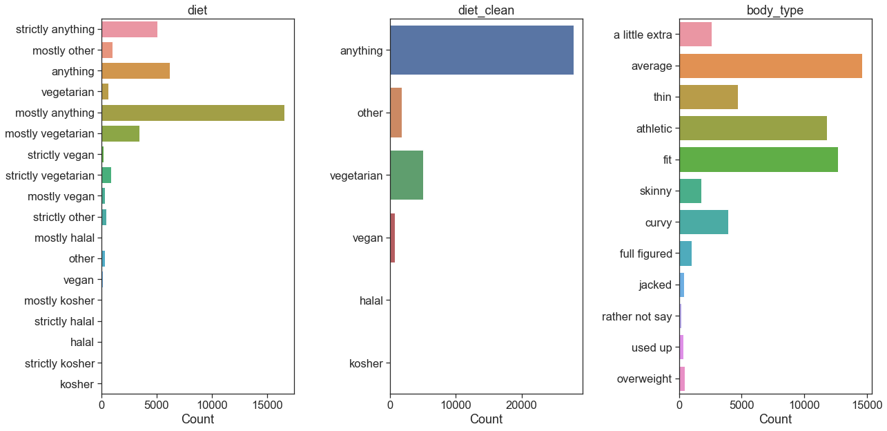
f, ax=plt.subplots(figsize=(15,6))
sns.color_palette("Spectral", as_cmap=True)
ax = sns.countplot(data=okc, x = 'body_type', hue='diet_clean')

ax.set_title('Distribution of dietary choices among different body types')
plt.xticks(rotation=20)
plt.xlabel('Body type')
plt.ylabel('Count')
plt.show()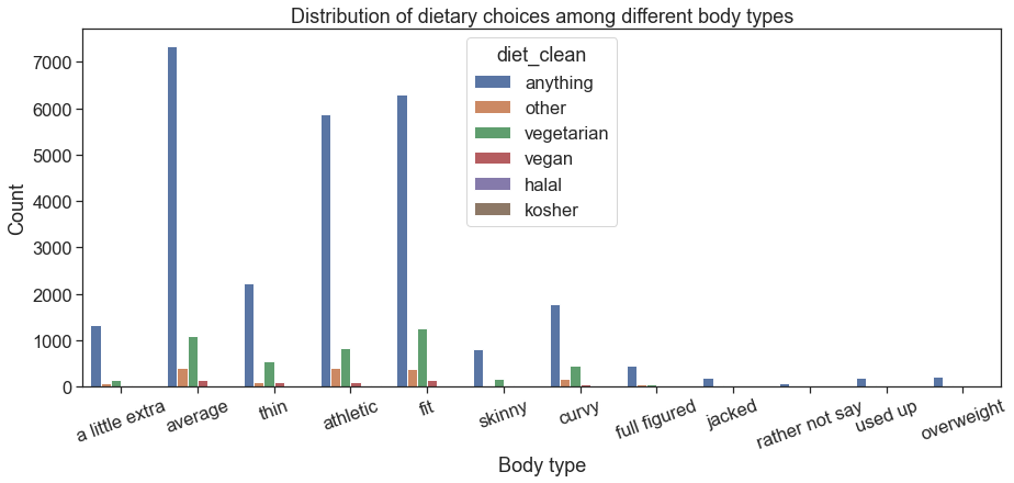
The majority of users are omnivores, with the next most prevalent choice being vegetarian. This is reflected in the relationship between diet and body type, with the majority dietary choice of each body type being omnivore and the second being vegetarian.
Lifestyle choices
Could a users smoking, drinking and drug habits be influenced by their zodiac sign?
lifestyle_choices = ['smokes', 'drinks', 'drugs']
plotting_tool(okc, lifestyle_choices, 20, 6)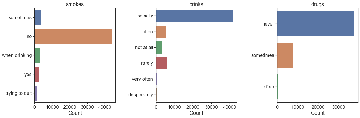
non_smoker = (okc.smokes == 'no').value_counts()
smoke_percent = round((non_smoker[1] / (non_smoker[1] + non_smoker[0])) * 100, 2)
social_drinker = (okc.drinks == 'socially').value_counts()
drinker_percent = round((social_drinker[1] / (social_drinker[1] + social_drinker[0])) * 100, 2)
uses_drugs = (okc.drugs == 'never').value_counts()
drugs_percent = round((uses_drugs[1] / (uses_drugs[1] + uses_drugs[0])) * 100, 2)
print(f'Percentage of users that drink socially {drinker_percent}%')
print(f'Percentage of users that never use drugs {drugs_percent}%')
print(f'Percentage of users that do not smoke {smoke_percent}%')
Percentage of users that drink socially 69.7%
Percentage of users that never use drugs 62.93%
Percentage of users that do not smoke 73.23%The data shows that the majority of users (~ 70 %) drink socially, do not use drugs or smoke.
Education and employment
attrib2=['education', 'job']
plotting_tool(okc, attrib2, 20, 10)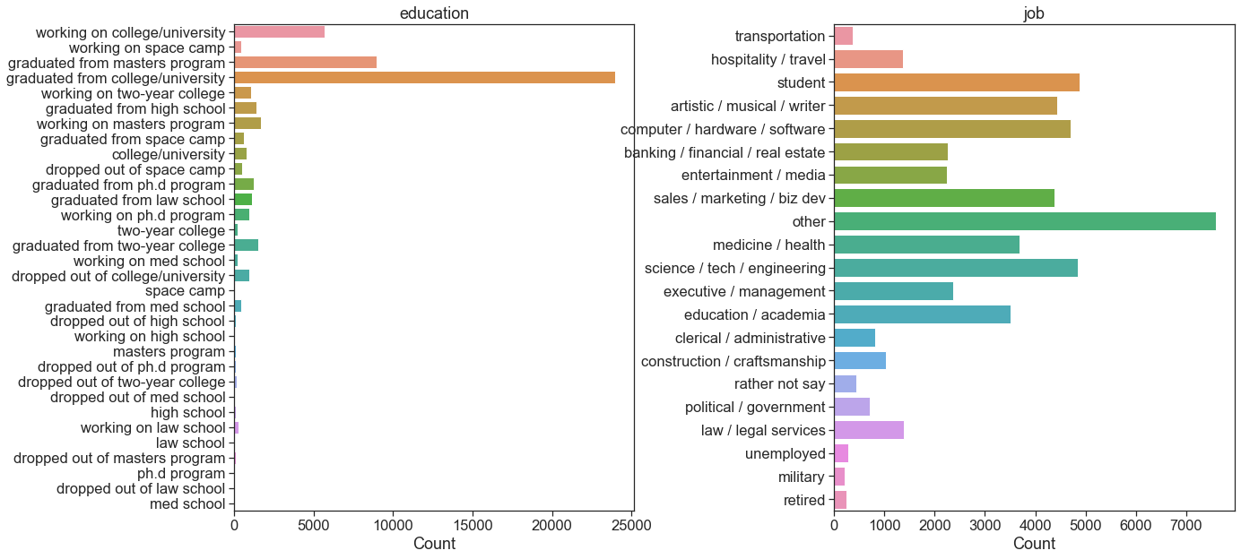
#collapse_output
print(okc.education.value_counts())
graduated from college/university 23959
graduated from masters program 8961
working on college/university 5712
working on masters program 1682
graduated from two-year college 1531
graduated from high school 1428
graduated from ph.d program 1272
graduated from law school 1122
working on two-year college 1074
dropped out of college/university 995
working on ph.d program 983
college/university 801
graduated from space camp 657
dropped out of space camp 523
graduated from med school 446
working on space camp 445
working on law school 269
two-year college 222
working on med school 212
dropped out of two-year college 191
dropped out of masters program 140
masters program 136
dropped out of ph.d program 127
dropped out of high school 102
high school 96
working on high school 87
space camp 58
ph.d program 26
law school 19
dropped out of law school 18
dropped out of med school 12
med school 11
Name: education, dtype: int64There are a lot of options within the education column, with the majority of answers indictating users graduating from or attending college/university. As the variable is dominated by people attending/completing college, it will not be used within the model. It is of note that space camp seems to be strangely popular. There is a range of employments, with no one industry dominating the answers, therefore this will be included in the model.
Pets and orientation
rel_status = ['status', 'orientation']
plotting_tool(okc, rel_status, 20, 6)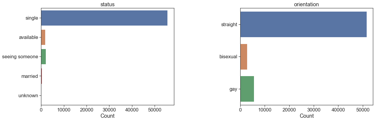
single = (okc.status == 'single').value_counts()
single_percent = round((single[1] / (single[1] + single[0])) * 100, 2)
print(f'The percentage of users that are single: {single_percent} %')
straight = (okc.orientation == 'straight').value_counts()
straight_percent = round((straight[1] / (straight[1] + straight[0])) * 100, 2)
print(f'The percentage of users that identify as straight: {straight_percent} %')
The percentage of users that are single: 92.91 %
The percentage of users that identify as straight: 86.09 %93% of users identify as single, which is unsurprising as OkCupid is a dating site. OkCupid also lets people identify as polyamorous or in open relationships, which accounts for the 7% that are not single. As the ‘single’ result dominates the answers, the relationship status variable will not be used in the model. A poll in the US on sexual orientation 3 found that 7.1% of people identified as LGBT. The OkCupid data shows 14% of people identify in this category. As this is twice the poll average it may be of benefit to the model so orientation will be included.
pet_status = ['pets']
plotting_tool(okc, pet_status, 10, 6)
children_status=['offspring']
plotting_tool(okc, children_status, 10,6)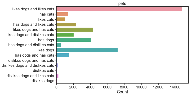
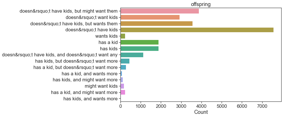
Most users appear to like both cats and dogs, with those liking dogs making up the second most popular answer. Most people do not have children (with qualifying information whether they want them in the future or not). Given the average age and the fact it is a dating site, it is unsurprising most people do not have children. The offspring data will not be included in the model as it is not easily simplified, thus making it hard for the model to learn anything from.
Religion
print('Cleaning the data to remove the qualifying information')
okc['religion_clean'] = okc.religion.str.split(' ').str[0]
#print(okc.religion_clean)

reli = ['religion', 'religion_clean']
plotting_tool(okc, reli, 20, 15)
Cleaning the data to remove the qualifying information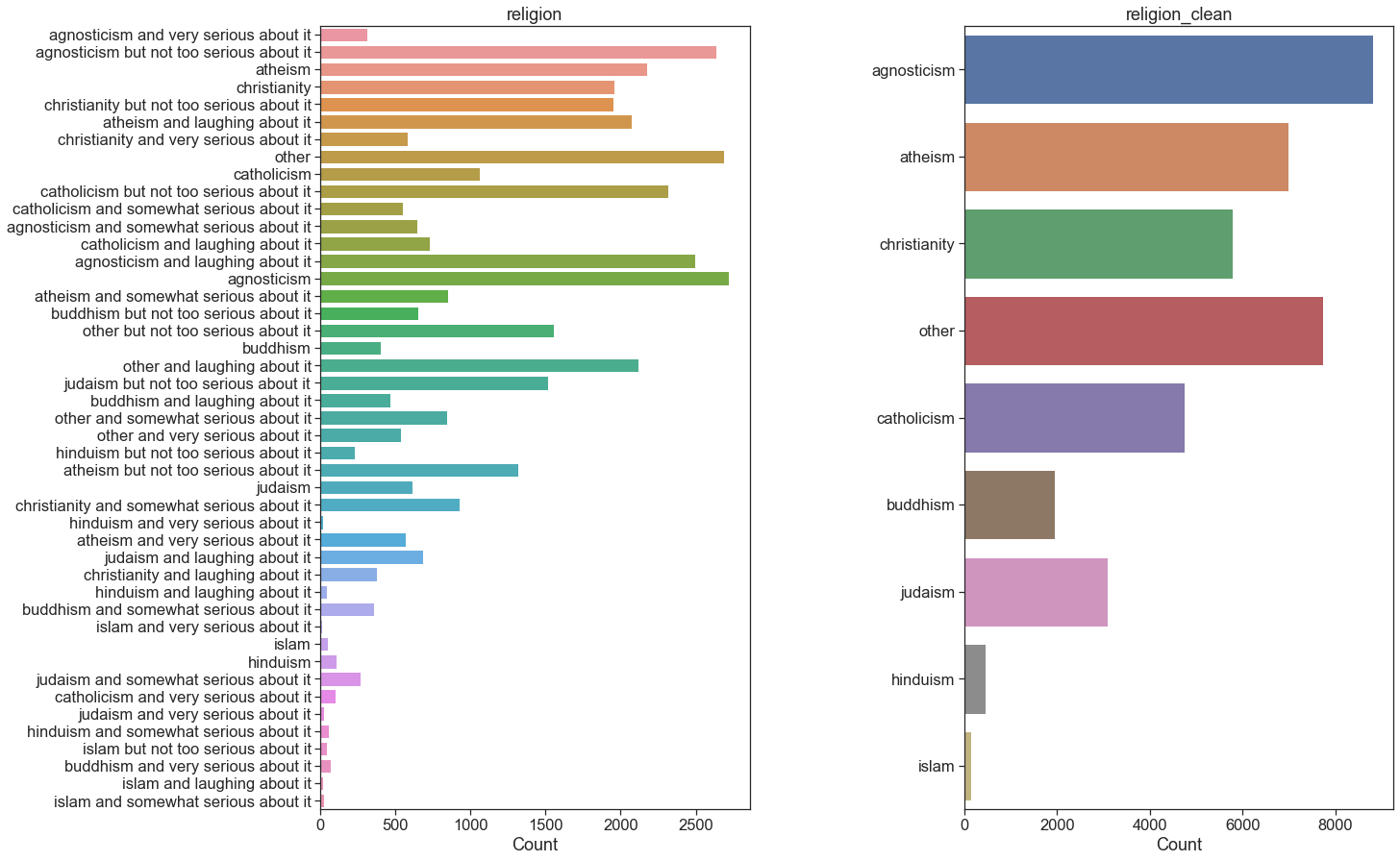
As with the zodiac data, the religion column also contains qualifying information. The data has been cleaned into a new column religion_clean to remove the qualifying data. There seems to be a spread of religions, with no one answer dominating the data.
Data preparation
Preprocessing
columns_for_model = ['body_type', 'diet_clean', 'job', 'pets', 'religion_clean', 'orientation', 'sex', 'sign_clean']
print(len(okc.diet_clean))59944Number of null values in each column
nulls = (okc[columns_for_model].isnull().sum(axis = 0))
print(nulls)

nulls_values = []

for null in range(len(nulls)):
    nulls_values.append(nulls[null])
print(nulls_values)
body_type 5295
diet_clean 24394
job 8197
pets 19919
religion_clean 20225
orientation 0
sex 0
sign_clean 11055
dtype: int64
[5295, 24394, 8197, 19919, 20225, 0, 0, 11055]Producing a dataframe of values
null_comb = list(zip(columns_for_model, nulls_values))
print(null_comb)

null_df  = pd.DataFrame(null_comb, columns=['Column', 'NaN'])


null_df['% NaN values'] = round((null_df.NaN / (len(okc))) *100, 2)
display(null_df)
[('body_type', 5295), ('diet_clean', 24394), ('job', 8197), ('pets', 19919), ('religion_clean', 20225), ('orientation', 0), ('sex', 0), ('sign_clean', 11055)]| Column | NaN | % NaN values | |
|---|---|---|---|
| 0 | body_type | 5295 | 8.83 |
| 1 | diet_clean | 24394 | 40.69 |
| 2 | job | 8197 | 13.67 |
| 3 | pets | 19919 | 33.23 |
| 4 | religion_clean | 20225 | 33.74 |
| 5 | orientation | 0 | 0.00 |
| 6 | sex | 0 | 0.00 |
| 7 | sign_clean | 11055 | 18.44 |
The null values within the data need to be addressed. As the model will be looking at zodiac signs, the NaN values in the sign_clean column are best removed. As there are not a large number of null values (9% and 14%, respectively) in the body_type and job columns, these null values will also be dropped.
columns_to_remove_nan = ['sign_clean', 'body_type', 'job']
for n in columns_to_remove_nan:
    print(n)
sign_clean
body_type
jobdef remove_nulls(df, cols, df_columns, df2):
remaining_null = []
for n in cols:
df = df.dropna(subset=[n])
drop_null = df[df_columns].isnull().sum(axis = 0)
for value in drop_null:
remaining_null.append(value)
df2[f'NaN after {n} null drop'] = pd.Series(remaining_null)
remaining_null = []
return df, df2okc_drop, null_df = (remove_nulls(okc, columns_to_remove_nan, columns_for_model, null_df))print(len(okc_drop))
display(null_df)40755| Column | NaN | % NaN values | NaN after sign_clean null drop | NaN after body_type null drop | NaN after job null drop | |
|---|---|---|---|---|---|---|
| 0 | body_type | 5295 | 8.83 | 3938 | 0 | 0 |
| 1 | diet_clean | 24394 | 40.69 | 18770 | 16005 | 13995 |
| 2 | job | 8197 | 13.67 | 4961 | 4196 | 0 |
| 3 | pets | 19919 | 33.23 | 13717 | 12389 | 10446 |
| 4 | religion_clean | 20225 | 33.74 | 14130 | 12553 | 10488 |
| 5 | orientation | 0 | 0.00 | 0 | 0 | 0 |
| 6 | sex | 0 | 0.00 | 0 | 0 | 0 |
| 7 | sign_clean | 11055 | 18.44 | 0 | 0 | 0 |
If null values were removed from diet_clean, religion_clean and pets then a large chunk of the data would be removed (over 40%).
print(okc_drop.diet_clean.unique())
print(okc_drop.pets.unique())
print(okc_drop.religion_clean.unique())
['anything' 'other' 'vegetarian' nan 'vegan' 'halal' 'kosher']
['likes dogs and likes cats' 'likes cats' 'likes dogs and has cats' nan
'likes dogs and dislikes cats' 'has dogs' 'has dogs and dislikes cats'
'has dogs and likes cats' 'likes dogs' 'has cats' 'has dogs and has cats'
'dislikes dogs and has cats' 'dislikes dogs and dislikes cats'
'dislikes cats' 'dislikes dogs and likes cats' 'dislikes dogs']
['agnosticism' nan 'atheism' 'christianity' 'catholicism' 'other'
'buddhism' 'hinduism' 'judaism' 'islam']Therefore, the null values are replaced with ‘unknown’ as perhaps certain zodiac signs have no opinion on pets, dietary or religious choices.
okc_drop =okc_drop.fillna('unknown')print(okc_drop.diet_clean.unique())
print(okc_drop.pets.unique())
print(okc_drop.religion_clean.unique())['anything' 'other' 'vegetarian' 'unknown' 'vegan' 'halal' 'kosher']
['likes dogs and likes cats' 'likes cats' 'likes dogs and has cats'
'unknown' 'likes dogs and dislikes cats' 'has dogs'
'has dogs and dislikes cats' 'has dogs and likes cats' 'likes dogs'
'has cats' 'has dogs and has cats' 'dislikes dogs and has cats'
'dislikes dogs and dislikes cats' 'dislikes cats'
'dislikes dogs and likes cats' 'dislikes dogs']
['agnosticism' 'unknown' 'atheism' 'christianity' 'catholicism' 'other'
'buddhism' 'hinduism' 'judaism' 'islam']print(okc_drop[columns_for_model].isnull().sum(axis = 0))
okc_model_df = okc_drop[['body_type', 'diet_clean', 'job', 'pets', 'religion_clean', 'orientation', 'sex', 'sign_clean']]body_type 0
diet_clean 0
job 0
pets 0
religion_clean 0
orientation 0
sex 0
sign_clean 0
dtype: int64The data is now clear of null values.
Dummy variables
The categorical data is ordinal, in that it does not follow a particular ranking or order. Therefore, in order to prepare this data for use in the models, features will be converted into dummies.
features = ['body_type', 'diet_clean', 'job', 'pets', 'religion_clean', 'orientation', 'sex']

okc_dummies = pd.get_dummies(data=okc_model_df, columns=features)
display(okc_dummies)
#print(okc_dummies.info())| sign_clean | body_type_a little extra | body_type_athletic | body_type_average | body_type_curvy | body_type_fit | body_type_full figured | body_type_jacked | body_type_overweight | body_type_rather not say | ... | religion_clean_hinduism | religion_clean_islam | religion_clean_judaism | religion_clean_other | religion_clean_unknown | orientation_bisexual | orientation_gay | orientation_straight | sex_f | sex_m | |
|---|---|---|---|---|---|---|---|---|---|---|---|---|---|---|---|---|---|---|---|---|---|
| 0 | gemini | 1 | 0 | 0 | 0 | 0 | 0 | 0 | 0 | 0 | ... | 0 | 0 | 0 | 0 | 0 | 0 | 0 | 1 | 0 | 1 |
| 1 | cancer | 0 | 0 | 1 | 0 | 0 | 0 | 0 | 0 | 0 | ... | 0 | 0 | 0 | 0 | 0 | 0 | 0 | 1 | 0 | 1 |
| 3 | pisces | 0 | 0 | 0 | 0 | 0 | 0 | 0 | 0 | 0 | ... | 0 | 0 | 0 | 0 | 1 | 0 | 0 | 1 | 0 | 1 |
| 4 | aquarius | 0 | 1 | 0 | 0 | 0 | 0 | 0 | 0 | 0 | ... | 0 | 0 | 0 | 0 | 1 | 0 | 0 | 1 | 0 | 1 |
| 5 | taurus | 0 | 0 | 1 | 0 | 0 | 0 | 0 | 0 | 0 | ... | 0 | 0 | 0 | 0 | 0 | 0 | 0 | 1 | 0 | 1 |
| ... | ... | ... | ... | ... | ... | ... | ... | ... | ... | ... | ... | ... | ... | ... | ... | ... | ... | ... | ... | ... | ... |
| 59936 | virgo | 0 | 0 | 1 | 0 | 0 | 0 | 0 | 0 | 0 | ... | 0 | 0 | 0 | 0 | 0 | 0 | 0 | 1 | 1 | 0 |
| 59942 | leo | 0 | 0 | 0 | 0 | 1 | 0 | 0 | 0 | 0 | ... | 0 | 0 | 0 | 0 | 0 | 0 | 0 | 1 | 0 | 1 |
| 59943 | sagittarius | 0 | 0 | 1 | 0 | 0 | 0 | 0 | 0 | 0 | ... | 0 | 0 | 0 | 0 | 0 | 0 | 0 | 1 | 0 | 1 |
| 59944 | leo | 0 | 1 | 0 | 0 | 0 | 0 | 0 | 0 | 0 | ... | 0 | 0 | 0 | 0 | 0 | 0 | 0 | 1 | 0 | 1 |
| 59945 | gemini | 0 | 0 | 1 | 0 | 0 | 0 | 0 | 0 | 0 | ... | 0 | 0 | 0 | 0 | 0 | 0 | 1 | 0 | 0 | 1 |
40755 rows × 72 columns
Labels
The zodiac signs are the labels for the model so will be converted into numerical values.
okc_dummies['sign_labels'] = okc_dummies.sign_clean.astype('category').cat.codes
labels = okc_dummies[['sign_labels']]
labels_array = labels.squeeze().ravel()
print(labels_array)
[4 2 7 ... 8 5 4]Splitting the data
Import library to split the data for testing and training.
from sklearn.model_selection import train_test_splitThe data will be split 80% for training the model and 20% for validating the model.
X_data = okc_dummies.iloc[:, 1:-1]
y_data = okc_dummies.iloc[:, 0:1]


X_train, X_test, y_train, y_test = train_test_split(X_data, y_data, test_size=0.2, random_state=100)

print(X_train.shape)
print(y_train.shape)
print(X_test.shape)
print(y_test.shape)
(32604, 71)
(32604, 1)
(8151, 71)
(8151, 1)Converting the y data into an array.
y_train = y_train.to_numpy().ravel()
y_test = y_test.to_numpy().ravel()
Models
Logistic Regression
Logistic regression is a machine learning algorithm that predicts the probability (ranging from 0 to 1) of a datapoint belonging to a specific category. These probabilities are used to classify/assign the observations to the more probable group. An example of this is using a logistic regression model to predict the probability that an incoming email is spam. If the probability is greater than 0.5, the email could automatically be sent to the spam folder. The email is example is called binary classification as there are only two groups (i.e. spam or not spam).
As the zodiac data is not binary, a ‘multinomial’ argument can be passed to the model, so that it may classify more than 2 groups.
#import library
from sklearn.linear_model import LogisticRegression
from sklearn.metrics import classification_report, confusion_matrix
from sklearn.metrics import accuracy_score, recall_score, precision_score, f1_score
logres_model = LogisticRegression(max_iter=4000, multi_class='multinomial')
logres_model.fit(X_train, y_train)
logres_model.predict(X_test)
logres_test_score = logres_model.score(X_test, y_test)lr_perc_success = round(logres_test_score * 100, 2)
labels_chart = logres_model.classes_
print(lr_perc_success)8.5The model was only 8.5% successful in predicting a zodiac sign.
A confusion matrix is a tool that allows us to visualise the performance of a classification machine learning model. The matrix compares the actual target values with those predicted by the model.
#confusion matrix
conf_mat = confusion_matrix(y_test, logres_model.predict(X_test))
fig, ax = plt.subplots(figsize=(15,10))
sns.heatmap(conf_mat/np.sum(conf_mat), annot=True, fmt = '.1%', cmap = 'Spectral', xticklabels=labels_chart, yticklabels=labels_chart)
plt.xlabel('Predicted Features')
plt.ylabel('True Features')
plt.show()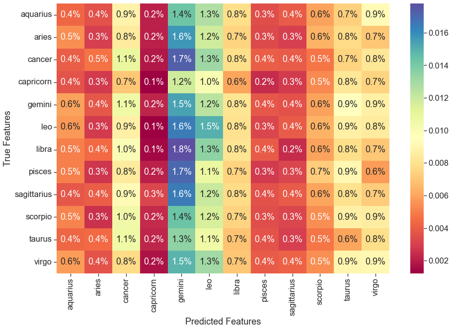
The above confusion matrix is showing that the model is unsuccessful in predicting any zodiac signs, with incorrect classifications across the board.
Logistic regression is generally used for continuous variable predictions not classification, therefore the lack of success above is unsurprising.
K-Nearest Neighbour (KNN)
KNN is a classification algorithm with central idea that data points with similar attributes tend to fall into similar categories. The KNN algorithm utilises this ‘feature similarity’ to predict the values of unknown/new data points. Therefore, a new point (or point from the test set) is assigned a value based on how closely it resembles the points in the training set.
from sklearn.neighbors import KNeighborsClassifierThe default number of neighbors within the algorithm is 5. As there are 12 zodiac signs, the model will initially be set to 12 nearest neighbors.
knn_model = KNeighborsClassifier(n_neighbors=12)
knn_model.fit(X_train, y_train)
predict_knn = knn_model.predict(X_test)
success_rate = knn_model.score(X_test, y_test)
print(round(success_rate * 100,2))8.7Like with the logistic regression model, the success at predicting a zodiac sign is between only 8 and 9 %. This is, again, highly inaccurate, so the measures of algorithm effectiveness are investigated below.
print(accuracy_score(y_test, predict_knn))
print(recall_score(y_test, predict_knn, average='weighted'))
print(precision_score(y_test, predict_knn, average='weighted'))
print(f1_score(y_test, predict_knn, average='weighted'))
0.08698319224635014
0.08698319224635014
0.08569285171615046
0.08313683542098019The accuracy, recall, precision and F1 scores are all between 8 and 9%, indicating that the KNN algorithm is highly ineffective in predicting a users zodiac sign.
Number of neighbours
The number of neighbors could affect the accuracy of the model. Therefore, the model will be run with number of neighbors from 1 to 100, to see if we can increase predictive accuracy, and also reveal the number of neighbors that gives the highest prediction success.
accuracy_values = []
for k in range(1,100):
    knn_model_neighbor = KNeighborsClassifier(n_neighbors=k)
    knn_model_neighbor.fit(X_train, y_train)
    accuracy_values.append(knn_model_neighbor.score(X_test, y_test))
#collapse_output
print(accuracy_values)
import altair as alt[0.08808735124524598, 0.08808735124524598, 0.0866151392467182, 0.08722856091277144, 0.08894614157772053, 0.08722856091277144, 0.08955956324377377, 0.08992761624340571, 0.09176788124156546, 0.08955956324377377, 0.08894614157772053, 0.08698319224635014, 0.08857808857808858, 0.08636977058029689, 0.0858790332474543, 0.08710587657956079, 0.08735124524598209, 0.08906882591093117, 0.08845540424487792, 0.0858790332474543, 0.08538829591461171, 0.08428413691571586, 0.08354803091645197, 0.08146239725187093, 0.08551098024782235, 0.08403876824929457, 0.0851429272481904, 0.085633664581033, 0.08416145258250521, 0.08391608391608392, 0.08403876824929457, 0.08317997791682002, 0.08575634891424365, 0.08502024291497975, 0.08710587657956079, 0.08624708624708624, 0.0866151392467182, 0.08600171758066495, 0.0868605079131395, 0.08624708624708624, 0.08502024291497975, 0.08281192491718807, 0.08317997791682002, 0.08170776591829224, 0.08452950558213716, 0.08428413691571586, 0.08170776591829224, 0.08293460925039872, 0.08121702858544964, 0.08354803091645197, 0.08391608391608392, 0.08477487424855847, 0.0848975585817691, 0.0848975585817691, 0.08477487424855847, 0.08440682124892651, 0.08416145258250521, 0.08551098024782235, 0.08551098024782235, 0.0848975585817691, 0.0858790332474543, 0.08600171758066495, 0.08477487424855847, 0.085633664581033, 0.08428413691571586, 0.08354803091645197, 0.08219850325113483, 0.08183045025150289, 0.08023555391976445, 0.0803582382529751, 0.08060360691939639, 0.0801128695865538, 0.08170776591829224, 0.08293460925039872, 0.08195313458471354, 0.08109434425223899, 0.08195313458471354, 0.08084897558581769, 0.0798675009201325, 0.07999018525334314, 0.08195313458471354, 0.08256655625076678, 0.08268924058397742, 0.08170776591829224, 0.08133971291866028, 0.08146239725187093, 0.08048092258618575, 0.08158508158508158, 0.08158508158508158, 0.08195313458471354, 0.08097165991902834, 0.08048092258618575, 0.0796221322537112, 0.07974481658692185, 0.07974481658692185, 0.08109434425223899, 0.08023555391976445, 0.08072629125260704, 0.07999018525334314]k_values = range(1,100)
knn_list = zip(k_values, accuracy_values)
knn_df = pd.DataFrame(knn_list, columns=['Number of neighbors', 'Model accuracy values'])
alt.Chart(knn_df).mark_line().add_selection(
    alt.selection_interval(bind='scales', encodings=['x'])


).encode(
    alt.X('Number of neighbors', type='quantitative', axis=alt.Axis(title='Number of neighbors', grid=False)),
    alt.Y('Model accuracy values', type='quantitative', axis=alt.Axis(minExtent=30, title='Model accuracy score', grid=False), scale=alt.Scale(zero=False)),
    tooltip=['Number of neighbors:Q', 'Model accuracy values:Q']


).properties(
    width=700,
    height=400
).configure_axis(
    labelFontSize=16,
    titleFontSize=20
).interactive()print(max(accuracy_values))0.09176788124156546The most successful prediction was 9.2%, with 9 nearest neighbors. This is still not a very successful model prediction, so another classification algorithm will be utilised.
Decision Tree
A decision tree model can be used to predict the class or value of a target variable by learning simple decision rules which are inferred from the training data. The number of trees is given by the n_estimators parameter.
from sklearn.ensemble import RandomForestClassifierforest_model = RandomForestClassifier(n_estimators=20)
forest_model.fit(X_train, y_train)
fmp = forest_model.predict(X_test)
print(forest_model.score(X_test, y_test))
print(forest_model.feature_importances_)0.08919151024414182
[0.01848739 0.02637059 0.03504928 0.01057379 0.02926258 0.01021325
0.00468601 0.00511136 0.00218385 0.01054881 0.02180001 0.00399913
0.03049809 0.00069427 0.0010625 0.01313826 0.02914841 0.00540481
0.01848554 0.02216242 0.01216928 0.00782094 0.01751775 0.00659331
0.01666686 0.01440667 0.01615785 0.01157835 0.0117934 0.01762815
0.00279926 0.02444587 0.00752194 0.00596421 0.00281248 0.01991651
0.01691888 0.01664402 0.00521809 0.00364966 0.00142563 0.00075272
0.00269392 0.00118054 0.00323092 0.01061822 0.02233436 0.00603287
0.01213355 0.01729834 0.00853359 0.02734466 0.01620145 0.01957317
0.03217913 0.03038652 0.02658916 0.01646818 0.0144284 0.01878572
0.01937051 0.00465989 0.00196257 0.01613154 0.02337304 0.02883307
0.01197838 0.01690925 0.02156606 0.01478103 0.01513981]Number of trees
The number of trees could affect the accuracy of the model. Therefore, the model will be run with number of trees from 1 to 100, to see if the model can increase predictive accuracy, and also reveal the number of trees that gives the highest prediction success.
accuracy_trees = []
for n in range(1,100):
    forest_model_trees = RandomForestClassifier(n_estimators=n)
    forest_model_trees.fit(X_train, y_train)
    accuracy_trees.append(forest_model_trees.score(X_test, y_test))
#collapse_output
print(accuracy_trees)[0.0858790332474543, 0.08317997791682002, 0.08575634891424365, 0.08771929824561403, 0.08391608391608392, 0.08305729358360937, 0.09495767390504233, 0.08722856091277144, 0.08342534658324131, 0.08747392957919274, 0.08551098024782235, 0.08845540424487792, 0.09422156790577843, 0.08870077291129923, 0.08919151024414182, 0.08673782357992885, 0.08636977058029689, 0.09066372224266961, 0.0866151392467182, 0.08649245491350754, 0.09090909090909091, 0.08870077291129923, 0.08673782357992885, 0.0913998282419335, 0.08796466691203533, 0.08931419457735247, 0.08980493191019506, 0.08747392957919274, 0.08992761624340571, 0.08771929824561403, 0.08821003557845664, 0.08354803091645197, 0.08894614157772053, 0.08636977058029689, 0.08931419457735247, 0.0911544595755122, 0.09348546190651454, 0.08747392957919274, 0.08747392957919274, 0.08919151024414182, 0.08845540424487792, 0.08882345724450988, 0.08943687891056312, 0.08882345724450988, 0.08919151024414182, 0.08673782357992885, 0.08636977058029689, 0.08796466691203533, 0.08980493191019506, 0.08354803091645197, 0.08722856091277144, 0.08710587657956079, 0.08808735124524598, 0.0851429272481904, 0.08931419457735247, 0.08821003557845664, 0.08857808857808858, 0.08919151024414182, 0.08575634891424365, 0.0851429272481904, 0.0866151392467182, 0.0916451969083548, 0.08857808857808858, 0.085633664581033, 0.08931419457735247, 0.08992761624340571, 0.08931419457735247, 0.08735124524598209, 0.0918905655747761, 0.08968224757698443, 0.08416145258250521, 0.08710587657956079, 0.0868605079131395, 0.08649245491350754, 0.08955956324377377, 0.08931419457735247, 0.08857808857808858, 0.08354803091645197, 0.08452950558213716, 0.08943687891056312, 0.08673782357992885, 0.08882345724450988, 0.08882345724450988, 0.0868605079131395, 0.08821003557845664, 0.08735124524598209, 0.08673782357992885, 0.09017298490982702, 0.08808735124524598, 0.08894614157772053, 0.08870077291129923, 0.08784198257882468, 0.0861244019138756, 0.09078640657588026, 0.09054103790945896, 0.08821003557845664, 0.08747392957919274, 0.08440682124892651, 0.08845540424487792]n_values = range(1,100)
#plt.plot(n_values, accuracy_trees)
#plt.show()tree_list = zip(n_values, accuracy_trees)
tree_list_df = pd.DataFrame(tree_list, columns=['Number of trees', 'Model accuracy values'])alt.Chart(tree_list_df).mark_line().add_selection(
alt.selection_interval(bind='scales', encodings=['x'])
).encode(
alt.X('Number of trees', type='quantitative', axis=alt.Axis(title='Number of trees', grid=False)),
alt.Y('Model accuracy values', type='quantitative', axis=alt.Axis(minExtent=30, title='Model accuracy score', grid=False), scale=alt.Scale(zero=False)),
tooltip=['Number of trees:Q', 'Model accuracy values:Q']
).properties(
width=700,
height=400
).configure_axis(
labelFontSize=16,
titleFontSize=20
).interactive()#collapse_all
print(accuracy_score(y_test, fmp))
print(recall_score(y_test, fmp, average='weighted'))
print(precision_score(y_test, fmp, average='weighted'))
print(f1_score(y_test, fmp, average='weighted'))0.08919151024414182
0.08919151024414182
0.08939718022369954
0.0891478760959913The decision tree model had no greater success than linear regression or k-nearest neighbor in predicting the zodiac sign of an OkCupid user, with all models having a success rate of > 10 %.
NLP and Naive Bayes
Naive Bayes classifiers are supervised machine learning algorithms that leverage a probabilistic theorem to make predictions and classifications. They are widely used for sentiment analysis (determining whether a given block of language expresses negative or positive feelings) and spam filtering.
Here a Naive Bayes classifier will be used to analyse the essay questions within the dataset to see if NLP has better success in predicting a users zodiac sign.
from sklearn.feature_extraction.text import CountVectorizer
import re
from nltk.tokenize import word_tokenize
from nltk.stem import PorterStemmer, WordNetLemmatizer
from nltk.corpus import stopwords
import nltk
#nltk.download('punkt')
#nltk.download('stopwords')
#nltk.download('wordnet')
Creating the dataframe and cleaning null values.
NB_df = okc[['sign_clean','self_summary', 'life_plans', 'good_at', 'notice_about', 'favourites',
             'do_without', 'think_about', 'friday', 'private', 'message']].copy()

#remove null values

NB_df = NB_df.dropna(subset=['sign_clean','self_summary', 'life_plans', 'good_at', 'notice_about', 'favourites',
                     'do_without', 'think_about', 'friday', 'private', 'message'])
print(NB_df.isnull().sum())
print(len(NB_df))
sign_clean 0
self_summary 0
life_plans 0
good_at 0
notice_about 0
favourites 0
do_without 0
think_about 0
friday 0
private 0
message 0
dtype: int64
26117Defining functions which utilise regex in order to clean the text, such as removing symbols and extra white spaces.
def regex_function(text):
    return re.sub('<.*?>|\\n+|http\S+|(?<=&)(.*?)(?=;)|,|\.|\:|;|-|/|&|!|\?|\(|\)|\+|@', ' ', text)

def remove_extra_whitespace(text):
    return re.sub(r'\s+', ' ', text)
essay_list = ['self_summary', 'life_plans', 'good_at', 'notice_about', 'favourites', 'do_without', 'think_about', 'friday', 'private', 'message']
for essay in essay_list:
NB_df[essay] = NB_df[essay].apply(lambda x: regex_function(x))
NB_df[essay] = NB_df[essay].apply(lambda x: remove_extra_whitespace(x))
NB_df[essay] = NB_df[essay].str.lower()(NB_df.head())| sign_clean | self_summary | life_plans | good_at | notice_about | favourites | do_without | think_about | friday | private | message | |
|---|---|---|---|---|---|---|---|---|---|---|---|
| 0 | gemini | about me i would love to think that i was some... | currently working as an international agent fo... | making people laugh ranting about a good salti... | the way i look i am a six foot half asian half... | books absurdistan the republic of mice and men... | food water cell phone shelter | duality and humorous things | trying to find someone to hang out with i am d... | i am new to california and looking for someone... | you want to be swept off your feet you are tir... |
| 5 | taurus | i'm an australian living in san francisco but ... | building awesome stuff figuring out what's imp... | imagining random shit laughing at aforemention... | i have a big smile i also get asked if i'm wea... | books to kill a mockingbird lord of the rings ... | like everyone else i love my friends and famil... | what my contribution to the world is going to ... | out with my friends | i cried on my first day at school because a bi... | you're awesome |
| 9 | cancer | my names jake i'm a creative guy and i look fo... | i have an apartment i like to explore and chec... | i'm good at finding creative solutions to prob... | i'm short | i like some tv i love summer heights high and ... | music my guitar contrast good food my bike my ... | you should | send a message | and say hi | you can rock the bells |
| 10 | taurus | update i'm seeing someone so off the market i ... | i have three jobs i've been doing sound and li... | hugging kissing laughing motivating people mas... | my huge goofy smile | i'm constantly reading i read at what my frien... | family friends food women music reading | snowboarding food women goofy nerd stuff archi... | having dinner and drinks with friends and or w... | i used to wish for a jetpack when blowing out ... | you are a complex woman with healthy self este... |
| 11 | leo | i was born in wisconsin grew up in iowa and mo... | i'm currently the youngest member on an intern... | i'm really good at a little bit of everything ... | the way i dress some days it's hats other days... | books = yes avid reader moves = eternal sunshi... | guitar even if i don't play it all the time i'... | a little bit of everything but mostly social i... | hanging out with a small group of friends stay... | i'm picky when it comes to dating i know what ... | if you know who you are who you want where you... |
Creating a dictionary of zodiac signs to map the dataframe to convert the signs into integers.
no_list = list(range(0,12))
print(no_list)
zodiac_list = list(okc_model_df.sign_clean.unique())
print(zodiac_list)
map_dict = dict(zip(zodiac_list, no_list))
print(map_dict)

#mapping the signs to integers
NB_df['sign_int'] = NB_df.sign_clean.map(map_dict)
(NB_df.head())
[0, 1, 2, 3, 4, 5, 6, 7, 8, 9, 10, 11]
['gemini', 'cancer', 'pisces', 'aquarius', 'taurus', 'sagittarius', 'leo', 'aries', 'libra', 'scorpio', 'virgo', 'capricorn']
{'gemini': 0, 'cancer': 1, 'pisces': 2, 'aquarius': 3, 'taurus': 4, 'sagittarius': 5, 'leo': 6, 'aries': 7, 'libra': 8, 'scorpio': 9, 'virgo': 10, 'capricorn': 11}| sign_clean | self_summary | life_plans | good_at | notice_about | favourites | do_without | think_about | friday | private | message | sign_int | |
|---|---|---|---|---|---|---|---|---|---|---|---|---|
| 0 | gemini | about me i would love to think that i was some... | currently working as an international agent fo... | making people laugh ranting about a good salti... | the way i look i am a six foot half asian half... | books absurdistan the republic of mice and men... | food water cell phone shelter | duality and humorous things | trying to find someone to hang out with i am d... | i am new to california and looking for someone... | you want to be swept off your feet you are tir... | 0 |
| 5 | taurus | i'm an australian living in san francisco but ... | building awesome stuff figuring out what's imp... | imagining random shit laughing at aforemention... | i have a big smile i also get asked if i'm wea... | books to kill a mockingbird lord of the rings ... | like everyone else i love my friends and famil... | what my contribution to the world is going to ... | out with my friends | i cried on my first day at school because a bi... | you're awesome | 4 |
| 9 | cancer | my names jake i'm a creative guy and i look fo... | i have an apartment i like to explore and chec... | i'm good at finding creative solutions to prob... | i'm short | i like some tv i love summer heights high and ... | music my guitar contrast good food my bike my ... | you should | send a message | and say hi | you can rock the bells | 1 |
| 10 | taurus | update i'm seeing someone so off the market i ... | i have three jobs i've been doing sound and li... | hugging kissing laughing motivating people mas... | my huge goofy smile | i'm constantly reading i read at what my frien... | family friends food women music reading | snowboarding food women goofy nerd stuff archi... | having dinner and drinks with friends and or w... | i used to wish for a jetpack when blowing out ... | you are a complex woman with healthy self este... | 4 |
| 11 | leo | i was born in wisconsin grew up in iowa and mo... | i'm currently the youngest member on an intern... | i'm really good at a little bit of everything ... | the way i dress some days it's hats other days... | books = yes avid reader moves = eternal sunshi... | guitar even if i don't play it all the time i'... | a little bit of everything but mostly social i... | hanging out with a small group of friends stay... | i'm picky when it comes to dating i know what ... | if you know who you are who you want where you... | 6 |
Creating a corpus column for use in model, in which all essay questions per row are joined into one string.
NB_df['corpus'] = NB_df[essay_list].apply(lambda row: ' '.join(row.values.astype(str)), axis=1)Writing the dataframe to csv, in order to check corpus is correct
NB_df.to_csv('NB_df1.csv')Preparing the data for use in Naive Bayes analysis, through definition of a function that will tokenize, stem and lemmatize the text, as well as removing stop words.
def NLP_processing(text):

    tokenized = word_tokenize(text)

    stemmer = PorterStemmer()
    stemmed = [stemmer.stem(token)for token in tokenized]

    lemmatizer = WordNetLemmatizer()
    lemmatized = [lemmatizer.lemmatize(token) for token in stemmed]

    stop_words = set(stopwords.words('english'))
    output = [x for x in lemmatized if x not in stop_words]

    output = ' '.join(output)

    return output
NB_df.corpus = NB_df.corpus.map(lambda x: NLP_processing(x))The data will be split into training and test sets before vectorizing - to avoid training data leaking into the test data. The data will be split 75% for training, 25% for testing.
corpus = NB_df.corpus
labels = NB_df.sign_int

NB_corpus_train, NB_corpus_test, NB_labels_train, NB_labels_test = train_test_split(corpus, labels, test_size=0.25, random_state=100)

print(NB_corpus_train.shape)
print(NB_labels_train.shape)
print(NB_corpus_test.shape)
print(NB_labels_test.shape)
(19587,)
(19587,)
(6530,)
(6530,)Creating and fitting the counter.
#hide-output
counter = CountVectorizer()
counter.fit(NB_corpus_train)CountVectorizer()In a Jupyter environment, please rerun this cell to show the HTML representation or trust the notebook.
On GitHub, the HTML representation is unable to render, please try loading this page with nbviewer.org.
CountVectorizer()
NB_train_counts = counter.transform(NB_corpus_train)
NB_test_counts = counter.transform(NB_corpus_test)
Creating and fitting the classifier
from sklearn.naive_bayes import MultinomialNBclassifier = MultinomialNB()
classifier.fit(NB_train_counts, NB_labels_train)
print(classifier.score(NB_test_counts, NB_labels_test))0.0888208269525268The model again has a success rate of ~ 9%, which is still disappointingly low. Below the confusion matrix will be utilised to see if the model was better at predicting some zodiac signs over others.
predictions = classifier.predict(NB_test_counts)
print(labels.value_counts(normalize=True))
matrix = confusion_matrix(NB_labels_test, predictions)
6 0.088410
0 0.088027
8 0.087989
1 0.086381
10 0.085117
4 0.083853
9 0.083394
7 0.083011
5 0.081977
2 0.079910
3 0.079488
11 0.072443
Name: sign_int, dtype: float64conf_mat2 = confusion_matrix(NB_labels_test, classifier.predict(NB_test_counts), normalize='true')
fig, ax = plt.subplots(figsize=(15,10))
sns.heatmap(conf_mat2/np.sum(conf_mat2), annot=True, fmt = '.1%', cmap = 'Spectral', xticklabels=zodiac_list, yticklabels=zodiac_list)
plt.xlabel('Predicted Features')
plt.ylabel('True Features')
plt.show()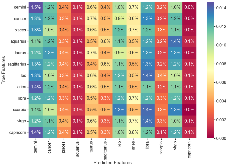
Again, the confusion matrix shows that the model is highly unsuccessful in predicting zodiac signs as it has struggled to make a distinction between any of the signs.
All the machine learning models above have failed to adequately predict zodiac signs. This will be discussed in the results and evaluation section below.
Evaluation
Results
The success of each machine learning algorithm, in predicting as OkCupid users zodiac sign were: - Linear Regression: 8.5 % - K-Nearest Neighbor: 9.1 % - Random Forest: 9.3 % - Naive Bayes: 8.9 %
All models have a success rate lower than 10%, which makes them all highly unsuccessful. Reasons for this, and suggestions for improvements are discussed below.
Conclusion
The goal of this project was to accurately predict the zodiac signs of OkCupid users from information provided in their profile through implementation of supervised machine learning classification models. Four different algorithms were utilised (linear regression, K-nearest neighbor, random forest and Naive Bayes classifier), with none achieving a success rate above 8-9 %. As there are 12 zodiac signs, a random guess has a 1 in 12 (or 8%) chance of being correct. This shows that a person guessing a zodiac sign has the same odds of guessing correctly as the machine learning model.
The conclusion we can take from this is that a person’s lifestyle choices and behaviours are not governed by their zodiac sign, meaning it is not possible to predict their zodiac sign from the data within a person’s OkCupid profile.
Next steps
This project could be further investigated by: - Obtaining a larger dataset, as with more information the models may have greater success in learning the difference between the features of the 12 classes. - As there are 12 zodiac signs, the number cannot be decreased. However the question posed to the ML model could be simplified/made binary i.e. Is a user a capricorn? - Are there better ways to preprocess or visualise the data? - Are there other aspects of the data a machine learning algorithm could investigate, such as can you predict a users sex, religion or drink/drug habits?